The 2D Scenario

In two dimensions, we deal with a flat surface where the points lie on a plane. The convex hull forms a polygon with vertices connected by straight line segments. We will begin by generating some random points and visualizing them using a scatter plot.

import matplotlib.pyplot as plt from scipy.spatial import ConvexHull import numpy as np

points = np.random.rand(20, 2) plt.plot(points[:, 0], points[:, 1], 'o') plt.xlim(0, 1) plt.ylim(0, 1) plt.gca().set_aspect("equal")

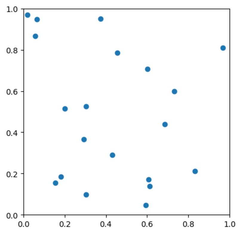
Next, we can compute the convex hull using the ConvexHull function from SciPy. This function employs the Quickhull algorithm and offers various attributes to visualize the convex hull.

hull = ConvexHull(points)

The vertices property gives the indices of the points that create the vertices of the convex hull.

hull.vertices array([ 5, 2, 18, 14, 6, 17, 0], dtype=int32)

The simplices property returns the indices of the points that form the simplicial facets of the convex hull. In two dimensions, these simplices are line segments connecting the vertices.

hull.simplices array([[ 2, 5],

[ 0, 5],

[ 0, 17],

[ 6, 17],

[ 6, 14],

[18, 14],

[18, 2]], dtype=int32)

Now, we will define a function to visualize the hull. The red circles indicate the vertices of the convex hull, while the red lines represent the segments forming the boundary.

def plot_hull():

plt.plot(points[:, 0], points[:, 1], 'o')

plt.plot(points[hull.vertices][:, 0], points[hull.vertices][:, 1], 'ro')

for facet in hull.simplices:

plt.plot(points[facet, 0], points[facet, 1], 'r-')

plt.xlim(0, 1)

plt.ylim(0, 1)

plt.gca().set_aspect("equal")

plot_hull()

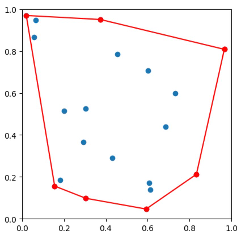
We can calculate the perimeter of the polygon through the area attribute of the hull object.

hull.area 3.142052162690126

The volume attribute refers to the interior of the hull, which in two dimensions equates to an area.

hull.volume 0.6449431389347489

To analyze neighboring facets of a given facet, we can use the neighbors property:

hull.neighbors array([[1, 6],

[0, 2],

[3, 1],

[2, 4],

[5, 3],

[4, 6],

[0, 5]], dtype=int32)

In this case, for facet 0, the neighboring facets are 1 and 6. For facet 1, the neighbors are facets 0 and 2, and so forth.

To demonstrate, we'll highlight facet 2 and its neighbors:

plot_hull()

# Highlight facet with index 2: facet = hull.simplices[2] plt.plot(points[facet].T[0], points[facet].T[1], 'g-', lw=3)

# Get indices of neighboring facets for hull vertex 2: neighbor_inds = hull.neighbors[2, :]

# Get point indices for ends of each neighboring facet: facets = hull.simplices[neighbor_inds] for facet in facets:

plt.plot(points[facet].T[0], points[facet].T[1], 'b-', lw=3)

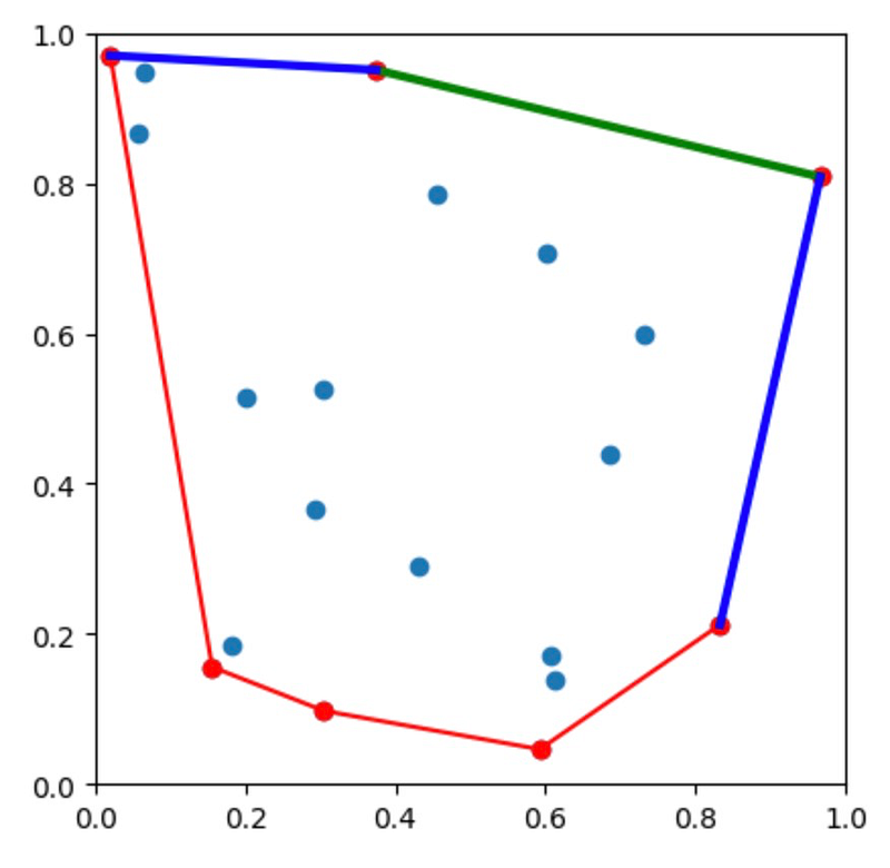
In the plot, facet 2 is displayed in green, while its neighbors are in blue.

The 3D Scenario

In three dimensions, the points exist in a 3D space, and the convex hull forms a polyhedron. The process for computing the convex hull is akin to the 2D case, although we now deal with three-dimensional facets and vertices.

from mpl_toolkits.mplot3d.art3d import Poly3DCollection points = np.random.rand(30, 3) hull = ConvexHull(points) fig = plt.figure() ax = fig.add_subplot(111, projection='3d')

# Plot the points ax.scatter(points[:, 0], points[:, 1], points[:, 2], 'o')

# Plot the convex hull vertices = [points[face] for face in hull.simplices] ax.add_collection3d(Poly3DCollection(vertices, facecolors='cyan', linewidths=1, edgecolors='r'))

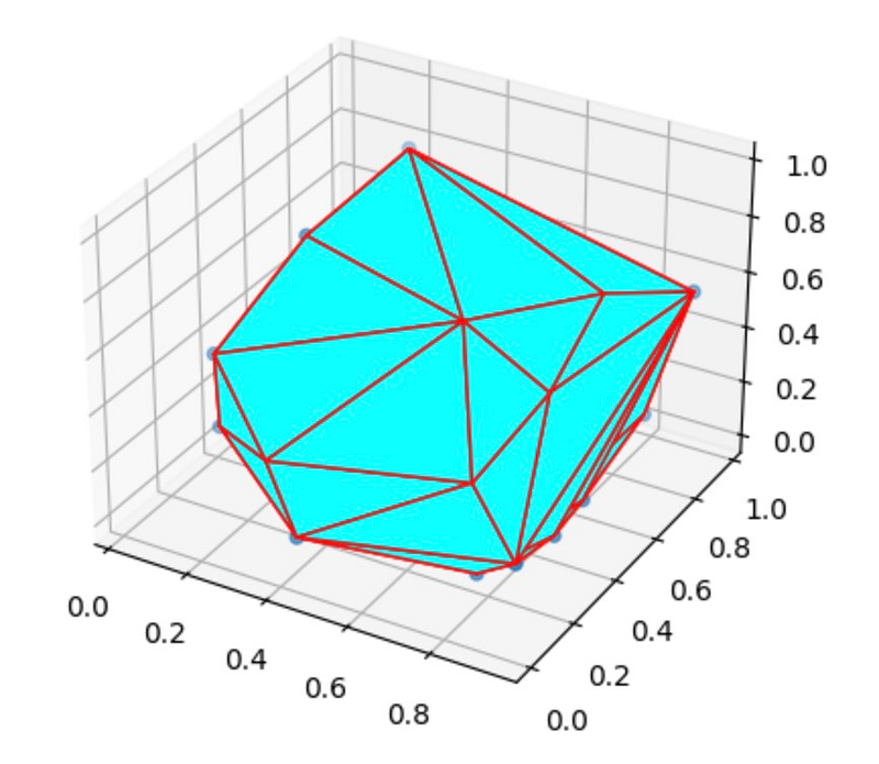
Here, we generated random 3D points and utilized SciPy’s ConvexHull function to compute the convex hull. The result is visualized as a polyhedron with cyan faces.

The vertices property in 3D indicates the indices of the points that form the vertices of the polyhedron.

hull.vertices array([ 0, 1, 3, 4, 5, 6, 7, 9, 10, 13, 14, 16, 19, 20, 21, 23, 25,

26, 27, 28, 29], dtype=int32)

The simplices property gives the indices of the vertices for each triangular facet of the convex hull.

hull.simplices array([[ 1, 9, 29],

[ 0, 25, 10],

[ 0, 19, 10],

[ 5, 19, 29],

[ 5, 19, 10],

[ 5, 1, 29],

[ 5, 1, 4],

[26, 1, 4],

[26, 1, 9],

[26, 3, 4],

[26, 3, 9],

[21, 0, 25],

[21, 25, 4],

[21, 3, 4],

[27, 5, 10],

[27, 5, 4],

[14, 6, 9],

[14, 9, 29],

[14, 19, 29],

[28, 3, 9],

[28, 6, 9],

[23, 0, 19],

[23, 14, 19],

[23, 14, 6],

[23, 0, 20],

[23, 6, 20],

[ 7, 21, 3],

[ 7, 0, 20],

[ 7, 21, 0],

[16, 25, 10],

[16, 27, 10],

[16, 25, 4],

[16, 27, 4],

[13, 7, 20],

[13, 7, 3],

[13, 6, 20],

[13, 28, 3],

[13, 28, 6]], dtype=int32)

To highlight a specific facet (with index 1):

fig = plt.figure() ax = fig.add_subplot(111, projection='3d') # Plot the points ax.scatter(points[:, 0], points[:, 1], points[:, 2], 'o') # Plot the convex hull vertices = np.array([points[face] for face in hull.simplices]) ax.add_collection3d(Poly3DCollection(vertices, facecolors='cyan', linewidths=1, edgecolors='r')) ax.add_collection3d(Poly3DCollection([vertices[1]], facecolors='green', linewidths=1, edgecolors='r'))

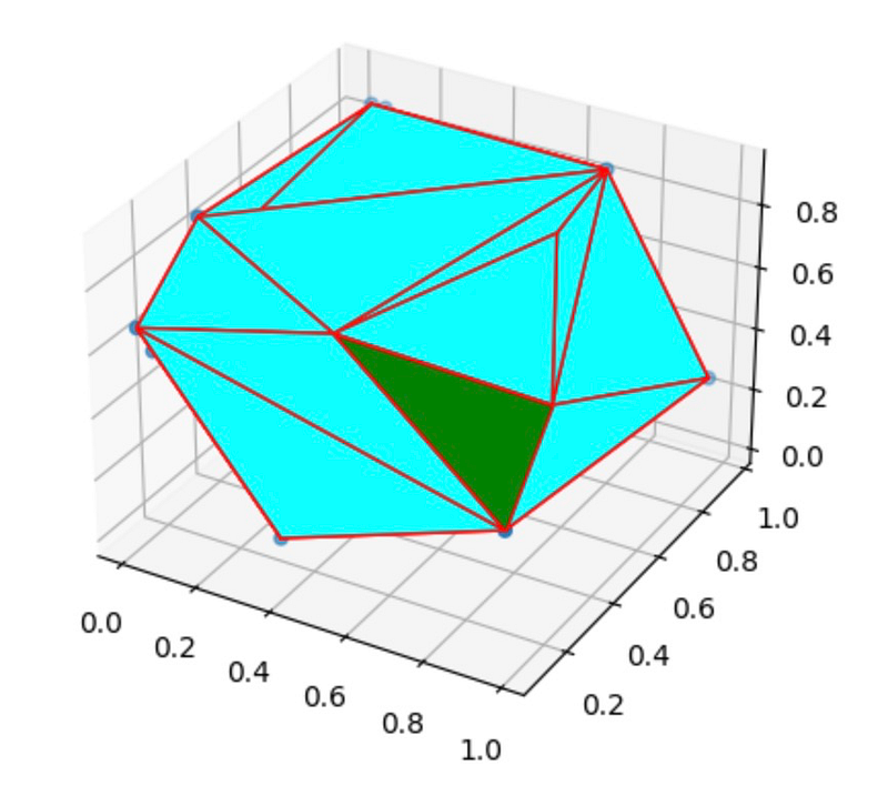
In this visualization, the facet with index 1 is highlighted in green, aiding in the analysis of specific hull components.

Conclusion

The concept of a convex hull is a cornerstone in computational geometry, with applications spanning computer graphics, pattern recognition, image processing, and optimization. This guide has demonstrated how to compute and visualize convex hulls in both 2D and 3D using Python's scipy.spatial package.

If you found this guide informative, consider becoming a Medium member for unlimited access to all Medium articles. Registering through this link also supports me as a writer.